
This work demonstrates the value of the results collected by RIPE Atlas independent of the original purpose for collecting them. Using all traceroute results from a particular day as an example, we first show that near real-time analysis of the result stream is feasible. Then we show that this has great potential for studying the packet layer of the Internet in general and for providing tools to network operators in particular. All this suggests a large and diverse potential for further work.
Introduction
One of the fundamental goals of RIPE Atlas is to provide a large collection of observations that can be used to study the IP layer of the Internet and to build tools to analyse the current state of it in near real-time. All measurements on RIPE Atlas contribute to this collection, independent of their individual purpose. Because the total number of observations is very large, this collection is expected to be useful in addition to the individual measurements. While we have stated this goal from the very beginning , little work has actually been completed. We will now demonstrate the potential of this existing collection of data and make suggestions for further work.
Background
RIPE Atlas provides a service to run active measurements. A measurement has a type , a target , a period and a number of sources often called ‘vantage points’ or simply ‘probes’. A result is the data obtained by observing the target from the source at a particular time. Each measurement produces one result from each source per period .
For example a typical traceroute measurement that uses 30 sources with a period of 15 minutes will produce an average of two results per minute. Each result contains the data obtained from running traceroute on one source towards the target with the parameters specified for the particular measurement .
The RIPE Atlas infrastructure collects and stores these results on a per measurement basis . In addition, RIPE Atlas provides streams of specific results for evaluation in near real-time. We recently added functionality to request a stream of all results of a specific type , independently of which measurement requested them.
The dataset
In order to demonstrate what can be achieved as a normal RIPE Atlas user without any special privileges we have set up a collection host located at about 12ms RTT from the RIPE NCC. The machine is a E5-1650 v3 Haswell with 128GB of RAM running Debian Linux. On this host we have installed RIPE Atlas Cousteau , a Python package for requesting RIPE Atlas data and RIPE Atlas Sagan for parsing this data.
We wrote a small python program that requests the stream and stores the results in a MySQL database. A number of small programs dump the results and perform basic analysis such as extracting data about each ‘hop’ recorded in the traceroute results.
We perform statistical analysis using RStudio . The reason for the generous amount of RAM installed is to facilitate easy and flexible analysis. Reading the stream does not require unusual amounts of memory. We have restricted ourselves to algorithms that could later be performed effectively on map/reduce architectures such as HADOOP.
The collection has been running since mid-April 2016. The data is available for bulk download . All results below are taken from the data collected for 24 consecutive hours starting on 1 May 2016 at 00:00 UTC.
Stream characteristics
We collected 37,562,853 results in the 24-hour period, an average of 26,085 per minute from a total of 9,408 different sources and belonging to 6,645 different measurements.
This is consistent with the number of results reported by the message queues that RIPE Atlas uses internally. The data stream is about 10Mbit/s on average. Looking at the whole period summarised per minute, the number of results received looks roughly as expected:

Figure 1: All RIPE Atlas traceroute results on 1 May 2016
However at a smaller scale the stream turns out the be quite bursty:

Figure 2: All RIPE Atlas traceroute results on 1 May 2016 - zoomed in
This burstiness and the observation that the single threaded receiving process sometimes hit 100% on one CPU core led us to suspect that there might be some losses. We therefore set up another independent collector machine and compared the received streams. Indeed, even after some code optimisations, both streams do not receive exactly the same results. Typically 99.7% of the results received on both streams are identical. Since our analysis will be based on ‘big numbers’ this presents no problem. However, it is important to bear in mind that two independent streams may not receive exactly the same results.
How old is the gold ?
Next we looked at the delay between the completion of the traceroute and the appearance of the result on the stream. We subtracted the timestamps generated by the probes from the timestamp of arrival on the collector. We can safely do that, because the clocks used to create these timestamps have been shown to be sufficiently accurate .

Figure 3: Delay between completion of the traceroute and the appearance of the result on the stream
This Cumulative Distribution Function (CDF) plot shows that half of all results are available on the stream about 90s after the traceroute starts and about 75s after it completes. It make little sense to wait for more than about four minutes for results.
For further analysis we discarded all results with timestamps in the future or more than four minutes in the past. This emulates data quality strategies that might be used when evaluating the stream in real time.
First sifting
In the next step we extracted individual ‘hops’ from all results received. Here is a listing of part of the data from a result in our dataset:
         1  192.168.1.1=0.9     192.168.1.1=0.7     192.168.1.1=0.7       priv 1


         2  217.13.80.129=1.1   217.13.80.129=1.0   217.13.80.129=0.9


         3  84.124.16.253=2.2   84.124.16.253=5.0   84.124.16.253=1.7


         4  10.254.12.101=2.7   10.254.12.101=2.2   10.254.12.101=2.2     priv 1


         5  10.254.0.66=1.8     10.254.0.66=1.8     10.254.0.66=1.8       priv 2


         6  10.254.8.85=2.0     10.254.8.85=2.1     10.254.8.85=1.9       priv 3


         7  10.254.10.118=1.6   10.254.10.118=1.7   10.254.10.118=1.6     priv 4


         8  212.162.42.9=1.8    212.162.42.9=1.7    212.162.42.9=1.8


         9  *                   *                   *                     star 1


         10 *                   *                   *                     star 2


         11 212.162.24.170=36.5 212.162.24.170=36.2 212.162.24.170=36.4


         12 *                   *                   *                     star 1


         13 188.43.18.97=109.8  188.43.18.97=109.5  188.43.18.97=109.6


         14 91.185.5.234=109.0  91.185.5.234=109.0  91.185.5.234=108.8


         15 91.185.20.62=121.8  91.185.20.62=120.3  91.185.20.62=120.3


         16 80.241.3.66=120.5   80.241.3.66=120.2   80.241.3.66=120.1
This traceroute took 16 ‘hops’ to reach the destination. The interface addresses in the rows denoted ‘priv’ are in private address space. The ‘hops’ with *s did not respond. In this example we saw responses from eight globally unique addresses and from five private addresses.
For this first analysis we use only the globally unique IP addresses of the interfaces that responded. We do not use all the other information, such as hop number, RTTs and the sequence in which the addresses occurred. In other words, we only count how frequently we saw a response from a particular globally unique address.
Our dataset contains responses from 511,353 globally unique IPv4 and IPv6 addresses. The Internet topology is not flat and our results are not from random paths. Therefore we expect to observe a small number of interfaces much more often than the vast majority. So let us look at the distribution of the most frequently observed addresses:

Figure 4: Interface addresses observed
Indeed this meets our expectations: the top 5% (25,568 addresses) are observed more than once per minute on average. The top 1.5% (7,670 addresses) are observed once every 10 seconds and the top 1% (5,114 addresses) are observed at least 10 times a minute.
What this means is that we can detect changes involving 25,568 interfaces within a couple of minutes and be fully aware of any change only three minutes after it occurs.
First nuggets
Next we sift through the observations for the interface addresses we observe most often. For this we use an extremely coarse and primitive sieve that only detects drastic changes by checking for major variations in the number of observations.
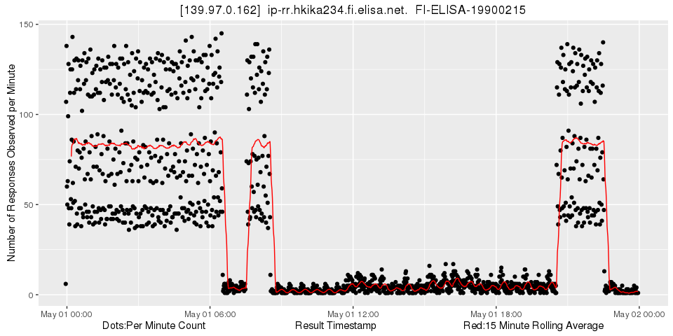
First we find 139.97.0.162:

Figure 5: Looking at 139.97.0.162
Obviously the number of observations changes abruptly here between two states. Zooming in shows that the 15 minute rolling average detects these changes very quickly while it fluctuates very little at other times:

Figure 6: Looking at 139.97.0.162 - zoomed in
15 minutes is the default period for traceroute measurements and also a common denominator of other popular period values. Note also that the rolling average only uses values observed in the past. This makes the method suitable for near real-time use.
Easily detecting a signal this strong is an encouraging result. Remember that we simply counted the occurrence of this address in our large but arbitrary selection of traceroute results. Of course the changes could be caused by huge and sudden changes in the measurements themselves. However, this is not so likely. In fact after just a little more sifting we find another nugget that complements our first one quite well:

Figure 7: Looking at 139.97.0.13
When we put both of these nuggets together we see that they fit nicely:

Figure 8: Combining 139.97.0.162 (blue) and 139.97.0.13 (red)
Using the same primitive sieve we find a major change in the Nordics:

Figure 9: Looking at various IPv4 addresses in the Nordics
This is paralleled in IPv6:

Figure 10: Looking at various IPv4 addresses in the Nordics
Since the sum of all observations increases after the event, it looks like our primitive sieve misses some of the interfaces involved before the change.
There is obviously more gold to be uncovered here and indeed we have found more interesting events even with our primitive ad hoc methods. It should be possible to detect more events and to interpret them automatically. With some cleverness we can envision reducing this to a stream of messages like:
      2016-05-01 06:23 elisa.net 139.97.0.162 -> 139.97.0.13


      2016-05-01 06:57 elisa.net 139.97.0.13 -> 139.97.0.162


      2016-05-01 09:12 nordu.net,netnod.se IPv4 multiple simultaneous changes


      2016-05-01 09:12 nordu.net,netnod.se IPv6 multiple simultaneous changes


      2016-05-01 09:12 nordu.net IPv6 increase
or
      2015-05-13 10:23:00 NL-AMSIX major drop


      2015-05-13 10:26:00 NL-AMSIX major drop continues


      2015-05-13 10:33:00 NL-AMSIX no longer observed !


      2015-05-13 10:41:00 NL-AMSIX observed again


      2015-05-13 10:42:00 NL-AMSIX major increase


      2015-05-13 10:44:00 NL-AMSIX major increase continues


      2015-05-13 10:46:00 NL-AMSIX at previous levels
Such a service, configurable and in near real-time could be quite useful for general situational awareness among network operators. Of course you will know much faster if something is wrong in your own network, but knowing what is going on around you and in areas of interest to your customers is quite valuable.
Second sifting
Next we look at what we can see if we do more than just count the number of times an address appears. We look at adjacencies. From our example
     1  192.168.1.1=0.9     192.168.1.1=0.7     192.168.1.1=0.7       priv 1


         2  217.13.80.129=1.1   217.13.80.129=1.0   217.13.80.129=0.9


         3  84.124.16.253=2.2   84.124.16.253=5.0   84.124.16.253=1.7


         4  10.254.12.101=2.7   10.254.12.101=2.2   10.254.12.101=2.2     priv 1


         5  10.254.0.66=1.8     10.254.0.66=1.8     10.254.0.66=1.8       priv 2


         6  10.254.8.85=2.0     10.254.8.85=2.1     10.254.8.85=1.9       priv 3


         7  10.254.10.118=1.6   10.254.10.118=1.7   10.254.10.118=1.6     priv 4


         8  212.162.42.9=1.8    212.162.42.9=1.7    212.162.42.9=1.8


         9  *                   *                   *                     star 1


         10 *                   *                   *                     star 2


         11 212.162.24.170=36.5 212.162.24.170=36.2 212.162.24.170=36.4


         12 *                   *                   *                     star 1


         13 188.43.18.97=109.8  188.43.18.97=109.5  188.43.18.97=109.6


         14 91.185.5.234=109.0  91.185.5.234=109.0  91.185.5.234=108.8


         15 91.185.20.62=121.8  91.185.20.62=120.3  91.185.20.62=120.3


         16 80.241.3.66=120.5   80.241.3.66=120.2   80.241.3.66=120.1
we can see that 217.13.80.12 appears before 84.124.16.253: (217.13.80.12, 84.124.16.253). So we can extract:
     (217.13.80.12, 84.124.16.253)


      (84.124.16.253, 212.162.42.9, 4p)


      (212.162.42.9, 212.162.24.170, 2s)


      (212.162.24.170, 188.43.18.97, 1s)


      (188.43.18.97, 91.185.5.234)


      (91.185.5.234, 91.185.20.62)


      (91.185.20.62, 80.241.3.66)
This way we extract information about the packet layer topology from our dataset. When we do that, again discarding results that arrive later than four minutes, we extract 347,605,342 such adjacencies. Each result provides about 10 adjacencies on average.
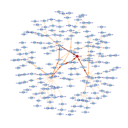
Let us look at the adjacencies to those NORDUnet IPv6 addresses involved in the major change we discovered earlier. Before the change (08:00-08:15 UTC) the adjacencies look like the image on the left in Figure 11:

Figure 11: Adjacenies to NORDUnet IPv6 addresses
The darker the arrow, the more often this adjacency is seen. After the change (10:00-10:15 UTC) it looks like the right image in Figure 11.
We can see that new paths via nl-sar.nordu.net are the major feature of the change. We do not know the reasons for this and whether this is due to a routing change or an anycast change. However, we know that a large number of paths have indeed changed at one specific time. There is a lot of room for further work here, like drawing this more nicely, finding the root cause of the change, etc.
In what neighbourhood is that ?
Often one wants to know in which ‘neighbourhood’ a specific address is located. The adjacencies discovered by RIPE Atlas traceroutes can help with that. Here is an example output of a simple command line tool that lets us see the neighbourhood of a specific address:
     ifrep -m 600 '2016-05-01 00:15' '2016-05-01 00:30' 213.207.0.226


      <     213.207.11.9                bitency.nikhef.jointtransit.nl   450


      <   217.170.11.217                 dommel.nikhef.jointtransit.nl   450


      <      213.207.3.1           nl-ix.nikhef.access.jointtransit.nl   225


      <   217.170.23.121               superior.nikhef.jointtransit.nl   180


      <    213.207.9.233         wirelessbelgie.nikhef.jointtransit.nl   180


      <    213.207.9.217                solidbe.nikhef.jointtransit.nl   150


      <   217.170.20.241                ipvisie.nikhef.jointtransit.nl   100


      <   217.170.20.129                kpn-nso.nikhef.jointtransit.nl    30


      <    217.170.19.73                 routit.nikhef.jointtransit.nl    29


      <    212.72.47.250       IPTRIPLEPLA.edge6.Amsterdam1.Level3.net     3


      <   176.56.179.137               4-4.r0.r327.nkf.ams.nl.iptp.net     3


      =    213.207.0.226           juniper-1.telecity2.jointtransit.nl     1


      >   217.170.19.204                       jointtransit.wide.ad.jp     1


      >    82.150.153.93         jointtransit.telecity2.openpeering.nl    18


      >   130.117.76.121     te0-0-0-19.agr21.ams03.atlas.cogentco.com    32


      >     213.207.8.92                         jointtransit.denic.de    40


      >   195.219.194.81 ix-xe-7-1-2-0.tcore1.AV2-Amsterdam.as6453.net    64


      >     213.207.8.36                      jointtransit-asd.kpn.com   150


      >     213.207.8.44                       jointtransit-rt.kpn.com   180


      >    62.115.145.74                         adm-b2-link.telia.net   450
In the first column ‘<’ means that the address appears one hop before the address of interest, ‘=’ is the address of interest and ‘>’ denotes addresses appearing one hop after the address of interest; the third column is the average number of seconds between observations of that address.
Conclusion
We have shown that there is a lot of useful information in the traceroute results collected by RIPE Atlas. Harvested properly, this information could provide unprecedented situational awareness to network operators about disturbances in the ‘neighbourhood’ and beyond. The information can also be used to augment traditional diagnostic tools such as traceroute with additional context.
Further work
There is a huge potential potential for clever anomaly detection and presentation. In fact some work has already been done with based on data dumps before the stream became available.
A lot of work can be done to eliminate experimental artifacts created by RIPE Atlas itself, such as probes going online and offline, experiments being started and stopped as well as those from measurements with many sources and long periods. Fluctuations in the stream of results itself need to be compensated too.
Some detailed questions that arose are:
-
Determine if privately addressed interfaces such as in rows 4-7 of the example traceroute result can be usefully interpreted, possibly based on the preceding and following hops.
-
Look at the beginning of the distribution of observed addresses. Why are some interfaces seen so infrequently? Is this due to some huge but infrequent measurements?
-
Which part of the Internet is covered by the frequently observed addresses?
-
How can one design additional measurements to monitor additional areas of interest?
This list is far from complete.
Resources
If you want to work on this data, the following resources from our lab may be useful. These are not RIPE NCC services.
Bulk download of results and adjacencies. This allows you to start looking at the data without investing in stream capture: ftp.labske.org
Snippets from code used to create this article: Github Repo
If you decide to work on this data, please do not hesitate to contact us.


Comments 0
The comments section is closed for articles published more than a year ago. If you'd like to inform us of any issues, please contact us.