Historical BGPlay

Historical BGPlay is a new tool developed by Claudio Squarcella, trainee at the RIPE NCC Science Group. Combining the power of the RIPE NCC's INRDB prototype and BGPlay, a routing visualisation tool developed at Claudio's home university Roma Tre, it shows the long term evolution of IPv4 and IPv6 prefixes, as seen by the Routing Information Service ( RIS ), over extended periods of time.

Introduction

You may have heard of the INRDB, the Internet Number Resource Database , which is a prototype service that stores and serves large amounts of historical data related to Internet number resources. It powers  REX, the resource explainer and it functions as a back-end database for a lot of research the RIPE NCC was performing lately. Currently it also stores the full RIS table dump history (10 years of routing data from multiple route collectors around the globe).

Many of you are also familiar with  BGPlay, a tool developed at Roma Tre University . BGPlay shows animated graphs with edges (peerings) connecting nodes (Autonomous Systems), allowing an intuitive analysis of interdomain routing events related to a specified prefix within a time interval. BGPlay can use recent routing events from  RIS or  RouteViews , and give insight into individual routing events.

My task was, as the topic of my master's thesis, to combine these tools and develop a new application that is more than just the sum of its parts . The result is a tool that lets us visualise the extended routing history related to any IPv4 or IPv6 prefix, during a specified, long time interval. The attention is focused on the dynamics of upstream ASes providing traffic towards any destination over an extended time period: in the order of weeks to months (or even years).

Getting Started

Historical BGPlay is available at  this link as a Java applet. Some recommendations:

• make sure you have the Java plugin ( version 1.5 or later ) available in your browser;
• being a prototype, the applet is  self-signed : if the browser warns you, just  accept the certificate.

How to Query

The new query interface is quite straightforward. It requires the user to specify the following fields:

• the desired  prefix , either IPv4 (a.b.c.d/e) or IPv6 (a:b:c:d:e:f/g). If it does not exactly match any record in the INRDB, the first available less specific prefix (if any) is silently chosen;
• the time interval of interest, bounded by  start and  end dates (yyyy-mm-dd);
• an optional  degree of filtering .

Figure 1: Query interface

As an example, in Figure 1 we are curious about  193.204.0.0/22 (prefix announced by Roma Tre University: the actual one is a  /15 , but BGPlay will not complain) during the  last year , with a specified filtering threshold of  two weeks . The result for the query (shown in Figure 2) is explained later.

Event Filtering

The last field in the query interface unveils one of the newly introduced concepts, going under the name of  event filtering . The underlying idea is that a historical analysis should only focus on  relevant events , namely those driven by real routing policy changes happened over time, ignoring  temporary events such as:

• disruptions or faults (e.g. undersea cable cuts);
• hijacked prefixes (e.g. 2008's  Youtube hijacking );
• temporary unavailability of RIS data.

Historical BGPlay comes with a  denoising system , which takes into account the specified  threshold interval as a reference value to discriminate between relevant and transient events. Some examples:

• when you just want to  get rid of fluctuations and limited route flapping , choose  low values (one or two days);
• if instead you specify a very large time interval you are probably willing to  look at the big picture : then choose  higher values (in the order of weeks) to concentrate on long-lasting routing policies, and the visualised graph will be cleaner and meaningful from a coarse-grained, historical point of view.

Main Features

The main interface is substantially identical to the one of the classical BGP update-based BGPlay:

• the routing graph and the time panel on the left are still the core of the applet;
• the upper part shows interesting textual data about visualised events and/or selected nodes in the graph;
• the control panel at the bottom allows the user to drive the animation, as well as to issue a new query.

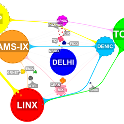
Figure 2: Main interface

Figure 2 shows the result for the example query listed above. Colored paths change in time, while dashed ones are stable; red nodes originate the prefix; ASes with numbers written in blue have direct peerings with RIS collectors, while those in black simply appear in one or more AS-paths. The animation can be intuitively controlled, either using the buttons at the bottom or clicking on the vertical timeline.

Despite the similarity, long time users will easily spot a couple of  colorful improvements . We walk through them focusing on the two main components of BGPlay: the  interactive graph and the  time panel .

Interactive Graph

After the layout is ready, the routing graph only shows a small number of nodes: namely, those representing Autonomous Systems which either originated the prefix ( origin ASes ) or had a direct peering with at least one originator ( upstream ASes ) at some point during the specified time interval. Disappointing? No worries. Just click on any visible node to reveal all the ASes that used it as a transit to reach the specified prefix. Click again to collapse it, reverting to the previous state. The reason is clear: since the Historical BGPlay potentially deals with far more complex topologies than its elder brother, it initially focuses on the immediate neighbourhood of the originating ASes , leaving the opportunity to expand/collapse nodes for a detailed analysis.

Figure 3: Expanded graph

Continuing with the proposed example, look at Figure 3 below. Some of the initially visible nodes are expanded; all connected nodes become visible, and in turn can be expanded (like AS2914, AS12956 and AS3058) to obtain a complete overview of a portion of the underlying graph.

Figure 4: Highlighted ASes

There is however a complementary way to highlight any desired Autonomous System. Want to know more about RIPE's AS? Simply type "3333" in the new text field on the right of the control panel and press Show/Hide AS : it will show up dressed in orange, together with all the other nodes involved in the routing paths toward the destination, if the visualised routing history contains information about it. Type any other AS number to highlight it; enter it again to go back (easy, isn't it?). See Figure 4 for details.

Time Panel

The new time panel is invaded by a handful of colored rectangles . What do they mean? Each one identifies a routing phase : that is, a time period in which all the inspected traffic goes through a specific set of upstream ASes. Now that rainbow stripe comes in handy - same color means same set of upstream ASes , so that two non-consecutive phases sharing the same configuration of active upstreams can be immediately distinguished. Want to know more? Hover a rectangle and the upstream ASes will appear, split between primary and secondary based on their overall activity period throughout the analyzed time interval. Cross proof: click on the left bar, let the graph show the routing state at that point in time, and observe the same set of active upstreams.

One last update. Highlighting one or more ASes (as described before) also lets some of the event peaks in the time panel stand out: each of them is a placeholder to immediately locate the instants when some changes affected the highlighted nodes - unless they were stable throughout the time interval.

Figure 5: Routing phases and highlighted events

Let's look again at Figure 4. The left bar is mainly dominated by yellow and blue routing phases, with a pale green interlude; when possible, the colors are arranged so that similar colors (in this case yellow and green) identify the same set of primary upstreams. Finally look at Figure 5, comparing it with the previous one: AS3356 ceases to provide connectivity during the blue routing phase, and the present stable routing state for the highlighted ASes remains unchanged after the last related event (yes, the orange spike!) on the vertical timeline.

So Long...

As usual, comments and feedback are welcome. Enjoy!

About the author:

Claudio Squarcella. Grad student in Computer Science at Roma Tre University.

Homepage: http://claudio.squarcella.com/