Bottleneck Bandwidth and Round-trip propagation time (BBR) is a congestion control algorithm (CCA) released for the Linux kernel by Google in 2016.

In a paper presented at the Internet Measurement Conference in Amsterdam in 2019, we provide the first model capturing BBR’s behaviour in competition with loss-based CCAs. Our model is coupled with practical experiments to validate its implications.

Modelling has been used in the past to understand a congestion control algorithm’s behaviour. For example, the Mathis equation showed TCP Reno’s throughput is inversely proportional to the loss-rate. In our research paper, we build a similar model to understand the flow of a BBR throughput when competing with other flows.

Our model has two important findings:

1. While BBR is supposed to be a rate-based algorithm, when competing BBR is window-limited. 
2. BBR’s throughput when competing with loss-based algorithms does not depend on the number of competing loss-based flows.

How does BBR work?

BBR is designed to be a rate-based algorithm. In contrast to window-based TCP variants (for example Cubic and Reno) which control the amount of in-flight data, BBR’s goal is to figure out what its fair share of the bottleneck link is and to pace sending packets at exactly that rate.

BBR determines the rate it’s going to send at by repeatedly probing for bandwidth (ProbeBW state). For 6 RTTs, BBR will send at whatever it currently thinks is the maximum throughput it can achieve. Then it’s going to try and put more data into the network to see if it can get better throughput. It does this by increasing its rate by 25% for 1 RTT. It may then observe that it can get a higher throughput than before. Finally, for 1 RTT, BBR will reduce its sending rate to what it now thinks is its maximum throughput. In total, these steps take 8 RTTs. BBR will repeat this 8 RTT cycle over and over again.

When 1 BBR flow is not sharing the bottleneck link with anyone, repeatedly probing for bandwidth allows BBR to both maximise throughput and minimise delay by figuring out exactly how much bandwidth is available.

But what happens during ProbeBW when BBR competes with Reno or Cubic?

During ProbeBW, BBR putting additional data into the network when the bottleneck link and queue are already full will cause packet loss. Because Reno and Cubic are loss-based algorithms, they will reduce their sending rates in response to packet loss. BBR on the other hand, will not reduce its rate; instead it will see that it was able to get better throughput and will increase its sending rate. This causes Reno and Cubic to end up with less bandwidth than BBR.

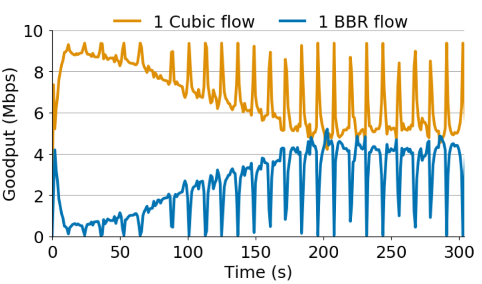
Figure 1: 1 BBR vs. 1 Cubic (10 Mbps network, 32 x bandwidth delay product queue).
During ProbeBW, BBR causes Cubic to back off

During ProbeBW, BBR will put more and more packets into the bottleneck queue, increasing its bandwidth estimate. This process will repeat over and over again. While the Cubic flows back off, BBR will push more and more packets into the queue. We can observe this behaviour shown in Figure 1.

Given what we know about BBR so far, during ProbeBW BBR should just keep putting more and more packets into the network until Cubic is starved. However, from Figure 1, we see that eventually BBR stops probing for more bandwidth.

Under competition, BBR is window-limited

Surprisingly, we find that under competition, BBR’s rate is not determined by its bandwidth estimate but by a window-limit called the in-flight cap.

BBR limits the amount of data in-flight to 2 BDP, as a safety mechanism in case of delayed and stretched ACKs. We find that this in-flight cap is what ultimately dictates what fraction of the link a BBR flow will get when competing with other flows and iswhat stops BBR during ProbeBW in Figure 1.

Therefore, if we can model the in-flight cap, we can figure out what BBR’s throughput will be when competing with loss-based flows.

A simple model for BBR’s throughput

To derive a simple model of BBR’s in-flight cap, and, consequently, its throughput, we assume that we have 1 BBR flow vs. any number of Cubic flows in a deep-buffered network (for example in Figure 1 the queue size is 32 BDP).

Figure 2: Variables in simple BBR model

First, let’s define some variables in the model shown in Figure 3. This illustrates what the bottleneck link and queue might look like. We assume the bottleneck link capacity is c and the bottleneck queue size is q. If the Cubic flows occupy p fraction of the queue, we assume that 1 BBR flow occupies the rest of the queue, (1-p) fraction.

Figure 3: A simple model for BBR’s queue occupancy/throughput. This model says 1 BBR flow can get up to half of the available queue/link capacity when competing with any number of Cubic flows.

Given this, we can draw a figure of Cubic’s queue occupancy vs. BBR’s, as shown in Figure 3. First, the blue line, 1-p, shows the amount of data inflight that BBR needs to occupy the rest of the queue next to the Cubic flows. 

Next, we need to model what BBR’s bandwidth and RTT estimates will be so we can also draw the 2 BDP inflight cap. BBR’s bandwidth estimate is equivalent to BBR’s fraction of the queue (which we have already said is 1-p) times the link capacity, which so it is (1-p)c. 

BBR determines its RTT estimate by continually tracking the minimal RTT it has seen over the last 10 seconds. Every 10 seconds, BBR goes into ProbeRTT state and lowers its inflight data to four packets so it can drain any of its packets from the queue and see what the minimum RTT is, minus any self-induced queue delay. Since BBR will drain its packets from the queue, the remaining packets in the queue will be Cubic. Thus, assuming a negligible propagation delay, BBR’s RTT estimate is going to be equivalent to Cubic’s queue occupancy divided by the link capacity so it is (pq) / c. 

Thus, BBR’s inflight cap = 2 * BW * RTT = (1-p)c * (pq)c = 2(p-p^2)q. This quadratic equation for the inflight cap turns out to be the green line in Figure 3. 

Returning to Figure 1, what we’re seeing is BBR moving up this blue line putting more and more data into the queue until the amount of data it has inflight meets its inflight cap. This intersection is illustrated in Figure 3 by the dashed orange line. This model shows that 1 BBR flow can get up to half of the link when competing with any number of Cubic flows! This is why we see unfairness between 1 BBR flow and 16 Cubic flows.

A more robust model for BBR’s throughput

Thus far, we have made many simplifying assumptions to make a simple model of BBR’s throughput. Our IMC paper builds a more complete model of BBR’s throughput when competing with any number of loss-based flows, relaxing those assumptions.

Figure 4: The robust model for BBR’s throughput/link fraction when competing with loss-based flows. Notably, none of the variables in the model depends on the number of loss-based flows.

One last note I’d like to mention relates to Figure 4, which highlights the variables that impact BBR’s fraction of the link and throughput. Notably, none of these variables depend on the loss rate or the number of loss-based flows. Consequently, BBR can be unfair to Cubic when there are more Cubic flows than BBR flows because the BBR flows aggregate fraction of the link will not be proportional to the number of flows.

The robust model can predict BBR’s throughput when competing against Cubic flows with a median error of 5% and 8% for Reno.

In summary, this model has two important explanations for why BBR can be unfair to Cubic:

1. While BBR is supposed to be a rate-based algorithm, when competing BBR is window-limited. As a result, although one of BBR’s goals is to minimise queueing delay, it will fill network buffers when competing with loss-based algorithms. 
2. BBR’s throughput when competing with loss-based algorithms does not depend on the number of competing loss-based flows. As a result, a single BBR flow will grab a fixed fraction of the link regardless of the number of competing flows.

Google recently proposed BBRv2 which aims to address the fairness issues discussed in this work and other fairness concerns by incorporating loss into BBR’s model of the network. BBRv2 is still in alpha, but after its official release, we aim to model the new approach to evaluate its fairness as we did for BBRv1.

If you’d like to know more, please watch our IMC presentation and read the full paper.