
Have you heard about MRT dumps, but never tried to use them because the bar seems too high? Or are you tired of doing “parse -> grep -> process” every time you touch BGP MRT dumps? This hands-on guide shows how to load RIS/RouteViews data into ClickHouse - covering tools, schema, and example queries - so you can explore prefixes, paths, and more with fast, ergonomic SQL.
Route collector projects - e.g. RIPE RIS, Routeviews, and others - collect BGP data in MRT files, a binary file format that can only be processed with specific programs. When working with such data, a common approach for many analysts is parse the raw MRT files for each new lookup they want to do: parse -> grep -> process.
This can be quite repetitive, but luckily, there are other ways. One alternative is to insert the data into a database and query that instead, making the whole process more ergonomic. Some people do this already, but there have been few write ups of how exactly to proceed.
To fix this, in this article we go through the basics of how you can index MRT data in ClickHouse in order to carry out your analysis. This isn't the only way to do this, and as indicated, we're relying on a specific infrastructure here. But we want to share this anyway because it gives a good illustration of a flexible approach that may well fit in your analysis stack. That said, if you're coming at this from a data science background, stay tuned: we plan to have a file format for that type of analysis ready by RIPE 91.
The following is a technical guide and assumes some familiarity with working with CLI commands and MRT files and performing standard queries for analysis. First, we'll go through the CLI commands for working with a dump file. After that, we will sketch the outline of how you can get the data into ClickHouse and how you query that.
Parse and Grep
The traditional way of working with MRT files is to use CLI tools for simple analysis, and use scripts/custom programs when you want to do a more complicated analysis. These tools usually parse the complete file for every analysis.
The benefit of this approach is that when you know what RIB/bview file you need to search in, or you are investigating the updates for a short time period, it is very fast to parse the files and filter the lines that you need. The example below uses bgpreader (from bgpstream). But you can also use monocle (from bgpkit).
$ bgpreader -m -d singlefile -o rib-file=bview.20250902.1600.gz | grep '193.0.14.0/24'
WARN: No time window specified, defaulting to all available data
TABLE_DUMP2|1756828800|B|80.77.16.114|34549|193.0.14.0/24|34549 25152|IGP|80.77.16.114|0|0|34549:200 34549:10000|NAG||
TABLE_DUMP2|1756828800|B|165.16.221.66|37721|193.0.14.0/24|37721 25152|IGP|165.16.221.66|0|0|37721:2000 37721:6002 37721:6003 37721:6004 37721:11000 37721:11100 37721:11101|NAG||
TABLE_DUMP2|1756828800|B|185.210.224.254|49432|193.0.14.0/24|49432 25152|IGP|185.210.224.254|0|1000||NAG||
TABLE_DUMP2|1756828800|B|193.33.94.251|58057|193.0.14.0/24|58057 1836 25152|IGP|193.33.94.251|0|0|1836:20000 1836:110 1836:3000 1836:3020 58057:65010 25152:1016|NAG||
...
Parsing MRT files in scripts
For a more complicated analysis you can write a script. There is a large number of libraries that parse MRT files (see this RIPE Labs article on the state of the art in 2018; and this RIPE 70 talk on CAIDA BGPStream). The libraries for parsing MRT files often have bindings for other languages, such as python, as well as CLI tools.
In a script you can do a more complex analysis. But, this has two downsides. The first is that you need to write a custom script, for which you need to know both a programming language as well as the library you are using. The second is that parsing takes time.
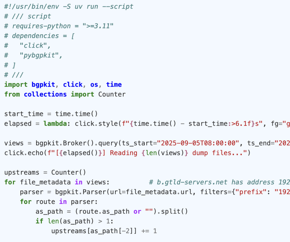
The next script counts the upstream AS's of k-root. When the files have already been downloaded, it takes around 20 minutes to run on my laptop:
#!/usr/bin/env -S uv run --script
# /// script
# requires-python = ">=3.11"
# dependencies = [
#   "click",
#   "pybgpkit",
# ]
# ///
import bgpkit, click, os, time
from collections import Counter

start_time = time.time()
elapsed = lambda: click.style(f"{time.time() - start_time:>6.1f}s", fg="green")

views = bgpkit.Broker().query(ts_start="2025-09-05T08:00:00", ts_end="2025-09-05T08:00:00", data_type="rib", project="riperis")
click.echo(f"[{elapsed()}] Reading {len(views)} dump files...")

upstreams = Counter()
for file_metadata in views:          # b.gtld-servers.net has address 192.33.14.30
    parser = bgpkit.Parser(url=file_metadata.url, filters={"prefix": "192.33.14.0/24"}, cache_dir=os.path.expanduser("~/.cache/bgpkit"))
    for route in parser:
        as_path = (route.as_path or "").split()
        if len(as_path) > 1:
            upstreams[as_path[-2]] += 1

print(f"[{elapsed()}] Results:")
for upstream, cnt in upstreams.most_common(10):
    print(f"  AS{upstream:<8} {cnt:>4}")
Loading BGP data in ClickHouse
Another approach is to use a database to store BGP data. That is what we are exploring in this article as another solution.
As a prerequisite for this, you need to have a ClickHouse database and the CLI tools working. This is out of scope for here, but there are tutorials online (ClickHouse website). The compose.yml file also gives an example of how to run ClickHouse (but not the client).
After that, the steps are
- Downloading MRT RIB dumps (or updates)
- Creating the table
- Parse and import the data
- Query ✨
Downloading MRT RIB dumps
You can download the MRT archives from https://data.ris.ripe.net/. Each collector has a directory (e.g. https://data.ris.ripe.net/rrc00/) in which there is a directory per month. For example one link for the rrc00 multi-hop collector is:
https://data.ris.ripe.net/rrc00/2025.09/bview.20250905.0000.gz.
When indexing in a database, I recommend to start with a low number of dumps to see how it performs in your environment. There are also tools to download dumps, e.g.:
$ uvx mrt-downloader ~/tmp/mrt/bviews \
  2025-09-02T16:00 \
  2025-09-02T16:00:01 \
  --rib-only \
  --project ris --project routeviews \
  --create-target
Downloading updates from 2025-09-02 16:00:00 to 2025-09-02 16:00:01 to /home/user/tmp/bviews
Partitioning directories by collector and month
Gathering index for 77 collectors: RRC00, RRC01, RRC02, RRC03, RRC04, RRC05, RRC06, RRC07, RRC08, RRC09, RRC10, RRC11, RRC12, RRC13, RRC14, RRC15, RRC16, RRC18, RRC19, RRC20, ...
This downloads all files in the time range (last second is exclusive). If you want only a specific collector, use --collector. For example --collector rrc13 for MSK-IX.
Creating the table
The tool that we will use here (monocle) has a pipe-separated output format. The table format may change depending on what you want to do. For this example I use:
CREATE TABLE rib
(
    `operation` String,
    `timestamp` DateTime,
    `peer_ip` String,
    `peer_as` String,
    `prefix` String,
    `as_path` String,
    `source` String,
    `next_hop` String,
    `_` String,
    `__` String,
    `communities` String,
    `___` String,
    `____` String,
    `_____` String,
    `______` String,
)
ENGINE = MergeTree
ORDER BY (prefix, peer_ip, peer_as)
This is the simplest schema possible. A more complicated version - an example of which I'll give at the end - might help reduce storage, make querying easier, etc. But for now, let's keep it simple :-).
Importing data
Importing data is quick and dirty. In this case:
- Use monocle (installation) to parse the file
- Use the ClickHouse CLI to connect to ClickHouse, set up the CSV separator, and load data from
STDIN.
The command below assumes you are in the directory where you downloaded the RIB files. It then parses each of them, configures ClickHouse to expect a | in CSV, and pipes the data into ClickHouse:
for bview in $(find . -name \*.gz); do
    monocle parse $bview | clickhouse-client --host=localhost --database=mrt --user=default --password=clickhouse -q "SET format_csv_delimiter = '|'; INSERT INTO rib FORMAT CSV"
done
Querying the DB
We finally have data available! We can now use it to analyse the default free zone. Many questions can be expressed in SQL. As a start, let's look up the announcements for a prefix:
SELECT *
FROM rib
WHERE prefix = '193.0.14.0/24'
LIMIT 2

Query id: 7ea7a828-987b-496e-8fe4-d886177ca741

   ┌─operation─┬───────────timestamp─┬─peer_ip────────┬─origin_as─┬─prefix────────┬─as_path─────────────────────────────┬─source─┬─next_hop───────┬─_─┬─__─┬─communities──────────────────────────────────────────────────────────────────────────────────────────────┬─___───┬─____─┬─_____─┬─______─┐
1. │ A         │ 2025-09-01 08:00:00 │ 86.104.125.108 │ 33823     │ 193.0.14.0/24 │ 33823 25152                         │ IGP    │ 86.104.125.150 │ 0 │ 0  │ 25152:1074 39107:25152 39107:650 39107:200 39107:500 25152:1074:39107 39107:39107:25152                  │ false │      │       │        │
2. │ A         │ 2025-09-01 08:00:00 │ 80.81.196.156  │ 34927     │ 193.0.14.0/24 │ 34927 59900 12297 201986 8932 25152 │ IGP    │ 80.81.196.156  │ 0 │ 0  │ 34927:130 34927:163 25152:1070:57463 57463:64700:25152 65000:0:100 65000:0:200 65000:0:202 65000:0:12297 │ false │      │       │        │
   └───────────┴─────────────────────┴────────────────┴───────────┴───────────────┴─────────────────────────────────────┴────────┴────────────────┴───┴────┴──────────────────────────────────────────────────────────────────────────────────────────────────────────┴───────┴──────┴───────┴────────┘

2 rows in set. Elapsed: 0.015 sec. Processed 270.27 thousand rows, 42.65 MB (18.16 million rows/s., 2.87 GB/s.)
Peak memory usage: 72.72 MiB.
Prefixes transiting an ASN:

SELECT
    countDistinct(prefix),
    multiIf(position(prefix, ':') > 0, 'ipv6', 'ipv4') AS afi
FROM rib
WHERE position(as_path, ' 1299 ') > 0
GROUP BY ALL

Query id: 5661cc1d-189d-4038-b536-d691ff0854e5

   ┌─countDistinct(prefix)─┬─afi──┐
1. │                211018 │ ipv6 │
2. │                965376 │ ipv4 │
   └───────────────────────┴──────┘

2 rows in set. Elapsed: 1.022 sec. Processed 443.89 million rows, 24.11 GB (434.54 million rows/s., 23.60 GB/s.)
Peak memory usage: 2.62 GiB.
This was a very simple first query. But SQL has many features that you can use. The only downsize is that - while database are vast - they are not magic. The data is still quite large, and ClickHouse also has to read all the columns that a query references.
The query planner helps a lot though. Depending on your query, the database may only need to read a small fraction of the rows in the database. Being a column-oriented database, it only reads the columns that you select. And, if you do aggregate queries (e.g. count), it may not even need to read the rows - it just has to know how many match.
Let's look at another query - a more complicated one. In this query we split the AS-path (from string into a list) and select the first upstream of the prefix. We then count how many announcements use this upstream:

Conclusion
Now you have a way to import BGP dump files into ClickHouse. It's a relatively simple way to work with MRT files, and it works. It works well. Queries are very fast when they match the order in which the data itself is stored.
There also is space for improvement: ClickHouse means infrastructure. And, because of the way the data is imported, it has little structure. AS paths are a string, which is both easy (you can do a regular expression) but also inefficient. We will give hints on some possible improvements in the appendix below.
ClickHouse works well when you continuously insert data into the database. There are many database systems available that you can use. My experience is that ClickHouse works quite well if you continuously insert new data.
If you can do your analysis on data that is older (for example: yesterday's BGP updates, yesterday's RIBs), the same queries can be possible on pre-processed files. Stay tuned for our presentation at the RIPE meeting on pre-processed files that offer an alternative to MRT for analysing BGP data.
In the future we will show more methods you can use to look at this data, including a workflow where we use joins to easily calculate statistics for multiple networks.
Improvements:
Earlier on I mentioned a number of possible improvements to the schema, a number of which are listed here and included in the updated schema and commands below. Be careful with every change that you do - they only help if the database or your queries use them.
- enum column for operation:
operation Enum8('A' = 1, 'W' = 2) LowCardinalitycolumn for dictionary encoding for columns with a low number of unique values (e.g.peer_ip)- Add secondary incides
INDEX prefixes prefix TYPE set(100) GRANULARITY 2 - order by truncated time to optimise queryies
ORDER BY (toStartOfFifteenMinutes(timestamp), prefix, peer_ip) - Partition the table
PARTITION BY toStartOfDay(timestamp)
CREATE TABLE rib
(
    `operation` Enum8('A' = 1, 'W' = 2),
    `timestamp` DateTime,
    `peer_ip` LowCardinality(String),
    `peer_as` LowCardinality(String),
    `prefix` String,
    `as_path` Array(String), --- recall: Can contain AS-sets
    `source` LowCardinality(String),
    `next_hop` String,
    `_` String,
    `__` String,
    `communities` Array(String),
    `___` String,
    `____` String,
    `_____` String,
    `______` String
)
ENGINE = MergeTree
ORDER BY (toStartOfFifteenMinutes(timestamp), as_path[-1], prefix)
PARTITION BY toStartOfDay(timestamp)
for bview in $(find . -name \*.gz); do
monocle parse $bview | clickhouse-client --host=localhost --database=mrt --user=default --password=clickhouse -q "
SET format_csv_delimiter = '|'; INSERT INTO rib
SELECT
operation, timestamp, peer_ip, peer_as, prefix,
splitByChar(' ', as_path_raw) as as_path,
source, next_hop, col9, col10,
splitByChar(' ', raw_communities) as communities,
col12, col13, col14, col15
FROM input('
operation String, timestamp DateTime, peer_ip String,
peer_as String, prefix String,
as_path_raw String,
source String, next_hop String, col9 String, col10 String,
raw_communities String, col12 String, col13 String, col14 String, col15 String
') FORMAT CSV"
done

Comments 0