
We've been working with various Internet Exchange Points (IXPs) over the last few months to see how RIPE Atlas active measurements can provide insight into how they are keeping local traffic local. This could help improve performance and efficiency for IXPs and their members. To explore this, we've created a set of Python scripts to analyse Internet traffic paths between RIPE Atlas probes in a given country and try to identify whether they traverse IXPs.
When measuring the interconnectivity of RIPE Atlas probes within a certain country, the simplest approach would be to just create traceroutes from each probe towards the public IP addresses of all the other probes. For countries with a small amount of probes this is certainly feasible.
For larger countries, you can select specific RIPE Atlas probes to do a more representative measurement. For instance, if a lot of probes are in a specific network (a very large access network, for example) or in a specific location, this will skew your results towards this network and/or location. I created a simple method to counter some of this bias, which will be used in the remainder of this article and is described below .
Keeping in-country traffic in-country
One way of measuring whether local traffic stays local is to check how many paths between end points in the same country we see going out of that country at some point along the path. Paths going out of a country are typically longer than paths staying in the country. The significance of going out of country may differ from country to country, but post-Snowden, country borders have gained importance - even while the Internet is, in principle, a globally connected network.
OpenIPMap
Because geolocation of IP addresses of network infrastructure is not a solved problem, we started OpenIPMap last year, to be able to crowdsource assigning geolocation to IP addresses. The current OpenIPMap prototype holds city-level geolocation information on over 30,000 IP addresses, mostly infrastructure IP addresses.
We used this information to see how many traceroute paths we observe going out-of-country. Note that OpenIPMap data doesn't completely cover all address space, and may contain inaccuracies, as any crowdsourced database does. Traceroutes also don't contain layer 1 and 2 information, so we don't know about the actual physical path, just the IP addresses and latency information that are exposed through traceroutes.
Example: Sweden
Since these measurements were first presented at the Netnod meeting last week in Stockholm, we looked at the situation in Sweden. All results below are based on a traceroute one-off mesh-measurement between 85 RIPE Atlas probes (out of 141 public probes), selected by their distance to Stockholm, Gothenburg and Kiruna as explained in the methodology below.
For IPv4, we observed out-of-country IP addresses in 12% of the paths. For IPv6, that was 21% .
Table 1 below shows a breakdown of specific countries that are seen in these paths.
| IPv4 | IPv6 | |
| DK | 7% (497) | 12% (107) |
| NO | 5% (352) | 5% (43) |
| NL | 0.4% (31) | 5% (51) |
| DE | 0.1% (7) | 5% (50) |
| GB | 0.2% (2) | |
| FI | 0.2% (2) |
Table 1: Specific countries seen in out-of-country paths between selected Swedish probes.
Figure 1 below shows the paths between all chosen RIPE Atlas probes for IPv4 and IPv6.

On our website you can find an animated interactive prototype of Figure 1. The interactive version uses animation to point out the directionality of the paths.
Traversing IXPs
From traceroute data we can infer whether traffic traverses an IXP. This is not an exact science, as ICMP return traffic might be blocked, but typically IXP peering LAN IPs are visible in traceroute paths. In this case I was interested in whether traffic traversed the various Netnod peering LANs. Note that this analysis can easily be redone with another IXP, or even a mix of IXPs.
For the set of Netnod peering LANs (north to south: Lulea, Sundsvall, Stockholm, Gothenburg and Malmö), 50.2% of paths traverse these peering LANs in IPv4, and 51.4% in IPv6.
Which peering LANs?
To look at path localisation at a sub-national level (for instance, whether paths between end points in the north stay in the north), I created the next visualisation. Credit to Kurtis Lindqvist for the idea. In the matrix in Figure 2 below, each row is a source probe and each column is a destination probe. Probes are ordered by latitude, north to south, with the most northern source-destination combination in the top left corner and the most southern source-destination combination in the bottom right corner. Cells are coloured by the IXP peering LAN that was seen between the source and destination probes.

On our website, you can find an animated interactive prototype of Figure 2. The interactive version allows you to see the actual traceroutes this information was derived from. This allows you to quickly zoom in to interesting traceroutes and also serves as a way to assess the quality of the data and analysis.
Figure 2 offers insight into which local traffic stays local. In this case, the Sundsvall LANs (blue) are seen in the north (top left), while the most southern exchange LANs in Malmö (orange) are seen mostly in the bottom-right corner. And the Gothenburg LANs (purple) are mostly seen above the Malmö LANs in Figure 2, which also makes sense geographically. The Stockholm LANs (green and red) are dominant, and they appear mostly in the centre, but also in the north and south.
It is also interesting to note that the 4470-MTU and 1500-MTU exchange LANs see 916 and 2,580 IPv4 paths respectively, an indication of their relative popularity.
IXP and in-country correlation
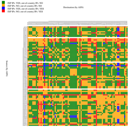
If IXPs help in keeping local traffic local, it is interesting to look at the correlation between a path going out-of-country and not traversing an IXP. In Figure 3, cells are coloured according to the following four combinations:
- Path via IXP, not going out-of-country (green)
- Path not via IXP, not going out-of-country (orange)
- Path via IXP, going out-of-country (blue)
- Path not via IXP, going out-of-country (red)
As seen in the figures above, paths dominantly stay within the country, either via IXP peering LANs (green), or without IXP peering LANs visible (orange). In the latter case, the IXP could still be involved, for instance through IXP-mediated private interconnects.

Again, you can find an animated interactive prototype of this figure on our website. The interactive version allows you to see the actual traceroute this information was derived from. This allows you to quickly zoom in to interesting traceroutes and also serves as a way to assess the quality of the data and analysis.
In cases where the path doesn't go via an IXP peering LAN and goes out-of-country (red), the IXP and/or the network operators involved could investigate whether it would make sense to consider alternatives to the current path. It could be by mistake that this path is taken, for instance due to a BGP misconfiguration. It could also be that optimising the paths between two Autonomous Systems (ASes) was never considered, for instance because traffic levels never reached the necessary threshold to appear on the radar of a peering coordinator. In that case, routing decisions can be reconsidered for economic reasons (traffic levels), but also for security and latency reasons. In bulk, these considerations can help an operator decide whether to connect to an IXP, or to start exchanging traffic with specific peers at an IXP.
Initially I was a bit puzzled by the small but still significant number of paths traversing an IXP but also going out-of-country (blue). Digging through the data, I noticed that Copenhagen and Oslo were the most frequent out-of-country cities.
I noticed that, for Stockholm-Gothenburg paths, Oslo was an intermediary hop in some of the backbone maps of operators I looked at, which could explain the prevalence of Oslo in the measured paths. Copenhagen is also easy to explain, as the Malmö peering LAN actually extends into Copenhagen.
With this local knowledge, I created a modified version of the IXP-out-of-country-correlation matrix (see Figure 4). In this case, I considered Copenhagen and Oslo as local to the Swedish Internet (only for the purpose of this analysis of course 😊), so paths that went Sweden-Oslo-Sweden or Sweden-Copenhagen-Sweden didn't count as out-of-country paths. Naturally this shows a different picture. Now the the image shows that the vast majority of paths between the RIPE Atlas probes in the Swedish Internet stay local (green and orange). For those few that don't, one could further investigate whether it makes sense to alter routing.

Figure 4: Same as Figure 3, but now considering Oslo and Copenhagen as in-country
Conclusion
I'm far from an expert in the Swedish interconnection space. Figures 3 and 4 show how having a flexible measurement and analysis platform allows this field to be explored. All the analysis shown in this article used a set of scripts that I put on GitHub as the IXP-Country-Jedi (alternative name suggestions welcome). This is my initial attempt to create a framework for targeted measurement campaigns using RIPE Atlas. It currently consists of a handful of scripts that are driven by a single config file needed to define which country and IXPs to watch. With this input, measurements are scheduled on RIPE Atlas and analysed. Finally, both textual representations and web-based visualisations of the recorded data are created. This is an open invitation to try out these scripts, and/or comment on how to improve its methodology, analyses and visualisations. If you know how to make this better, please comment below! Also, if people have created visualisations like this for a specific country and/or IXP, we'd be curious to see them.
Appendix: Probe Selection Methodology
Choosing a probe mesh
We set up traceroute measurements for both IPv4 and IPv6 between a set of RIPE Atlas probes in a country and with that created a mesh of traceroute measurements. We could have simply chosen all probes in one country, but that could potentially be very many, so we tried to select the set of probes based on the geographic location and the AS they live in. If we find probes in either the same AS or location, we assume they will produce redundant results.
The distribution of RIPE Atlas probes in a country is quite likely not a representative sampling of Internet end points in that country. And the paths between the probes are probably not the paths that carry the most traffic. For instance, in a radius of 30km from Amsterdam's centre, there are 165 probes. The top three ASes in the Netherlands host 42, 33 and 21 probes respectively. As probes in the same AS and location typically provide highly redundant information, we only need to select a single probe from a single location+ASN combination for a representative view of that AS in that location.
A variation would be to define a set of locations and, for each location, select both the farthest and closest probes within an AS.
For instance, to do a probe mesh traceroute for Sweden, which had a total of 141 public RIPE Atlas probes online at the time of measurement, I picked Stockholm, Gothenburg and Kiruna to try and get a probe sampling with reasonable location diversity. This resulted in a selection of 85 probes, covering 51 ASes, with at most six probes per AS.
This set of probes was used to do one-off traceroute measurements in IPv4 and IPv6 (when available).
Tag cloud
The RIPE Atlas interface allows probe hosts to add tags to their probes, such as "home", "NAT" and "data centre". This can be used by other RIPE Atlas users to filter probes when conducting their own measurements. The RIPE Atlas system itself also adds certain tags, such as the version number of the probe or whether the probe works over IPv6. In Figure 5 below, you can see the system tag cloud (top) and the tag cloud based on those tags set by probe hosts (bottom) for the probes selected for the measurements described above.

Figure 5: Tag cloud for selected RIPE Atlas probes in Sweden
A tag cloud like this can provide more insight into what is actually measured, and how to interpret the results of analysing and visualising the paths between selected probes. For instance, one can get a feel for the number of probes in a data centre versus probes located in people's homes.
Comments 4
The comments section is closed for articles published more than a year ago. If you'd like to inform us of any issues, please contact us.
Andrey Safonov •
Hi. While trying to measure traffic in Russia I'm getting the error "Executing this measurement request would violate your maximum daily spending limit of 1000000.0 credits. Please stop some of your currently running measurements and try again." How could I fix that?
Emile Aben •
Hi Andrey, Calculating back from this limit, it seems that the spending limit would be exceeded with 92 fully dual-stack probes. We do have a few countries with enough RIPE Atlas probes where this can be a problem (US,DE,RU) with the default maximum daily spending limit. One solution would be to change the scripts to select fewer probes, or only do one address family (IPv4 or IPv6), or to select maximum of 1 probe per ASN. Or you could manually modify the probeset.json file that gets generated and remove probes there yourself, to fit within the spending limit. I'll try and get back to you in direct email to get to know the details of the measurement you are attempting (for instance the number of locations specified, as that affects the number of probes). Tthe RIPE Atlas team can temporarily increase spending limits if there is a reason for that.
Cristian Espinosa •
I'm trying to work with the ixp-jedi tool. In this step: ## measure.py This script runs one-off measurements for the probes specified in _probeset.json_ and stores their results in _measurementset.json_ This uses the RIPE Atlas measurement API for measurement creation, And it needs a valid measurement creation API key in ~ / .atlas / auth When trying to execute the script ./measure.py I get the following and I do not know how to solve it. Authentication file /root/.atlas/auth not found Please, I need your help.
Emile Aben •
hi, thanks for trying to use the tool. i hope the docs on github are clear enough: https://github.com/emileaben/ixp-country-jedi/#measurepy --- This script runs one-off measurements for the probes specified in probeset.json and stores their results in measurementset.json This uses the RIPE Atlas measurement API for measurement creation, and it needs a valid measurement creation API key in ~/.atlas/auth . For more information on RIPE Atlas API keys see https://atlas.ripe.net/docs/keys/ --- if not let me know how to improve that. if you are interested in country-level monthy runs. these are available at: http://sg-pub.ripe.net/emile/ixp-country-jedi/history/