

Our VM pilot allows us an opportunity to run a like-for-like comparison between two RIPE Atlas anchors. We're grateful for the support from DigitalOcean, who are running two machines (one metal, one virtual) from the same geographical location.
Those anchors are:
- uk-slo-as202109.anchors.atlas.ripe.net (in this article, "anchor A")
- uk-slo-as14061.anchors.atlas.ripe.net (in this article, "anchor B")
They're located in different IPv4/IPv6 subnets and they're about 4 traceroute hops from each other, but they're only around 0.5ms apart from each other. This gives us a basis for comparison.
RIPE Atlas anchors participate in mesh measurements, which we've written about in the past. Both of the anchor pages above refer to the mesh measurements those anchors are participating in. For the purposes of this quick comparison, that's the data I'm borrowing for everything here, except the NTP measurements for which I scheduled one additional measurement. Seven days of data was taken from the ping and HTTP mesh measurements, commencing 20 June 2018 at 00:00 UTC.
Round-Trips
The mesh measurement data includes measurements from each anchor to all other anchors. That means that for both of the anchors we're discussing here, we have measurements from around 300 other anchors.
This permits a useful direct comparison: for each of those 300 measurements, we can take the difference between the two measured RTTs. That gives us a set of 300 deltas for every iteration of the measurement, which should give us an idea of whether one host is notably faster than the other.
RTT data is likely to be noisy, of course, but given these two anchors are based in the same geographic location and are topologically very similar locations the deltas ought to balance around 0ms. If the data shows a clear difference one way or another, we might be observing one host as being consistently faster or slower.
Here, I've taken ICMP echo requests (pings) and HTTP response times as two distinct round-trip measures that hit very different parts of the network stacks.
ping
The ping measurements iterate once every 240 seconds (4 minutes). First, this plot shows the median difference from each iteration, for IPv6 and IPv4:
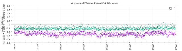

Figure 1: Median difference for ping measurements, for IPv6 (purple) and IPv4 (green)
Remember that this is showing the median delta from a range of values generated by pairs of vantage points, and if all else was equal all points would sit precisely on the 0ms line. Negative values indicate that one anchor ("anchor A") responded faster, and positive values indicate that the other anchor ("anchor B") responded faster.
It's clear that the median values do not sit on 0ms, but also it's clear that they're not forming a normal distribution around 0ms. The distinct trend is that, over these 7 days, anchor A responds around 0.25ms faster than anchor B over IPv6, and around 0.1ms faster over IPv4. That seems clear-cut, but we can look more broadly at the set of deltas to determine whether the trend is consistent.
The sets of offsets give us a range of values observed in the measurements. Latency distributions are heavy-tailed, so I'll take the 25th/75th percentiles (which will contain around 50% of the observed offsets) and the 5th/95th percentiles (which will contain about 90% of the observed offsets). Those offsets look like this:
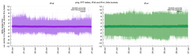

Figure 2: Percentiles for ping measurements
We see that these ranges do balance around 0ms, and that on the higher percentiles they skew differently to the median value alone.
- In the 25th/75th percentiles, the response times over IPv6 range from anchor A leading by around 0.9ms through to anchor B leading by around 0.6ms; over IPv4, that range is anchor A responding 0.8ms faster through to anchor B responding 0.4ms faster.
- In the 5th/95th percentile range, we see much more of the noise we'd expect in RTT data. Over IPv6, the 5th/95th percentile range indicates that anchor B can often respond 4-7ms faster than anchor A, and anchor A can often respond 3-5ms faster. On IPv4, those ranges are much wider. In both cases, the extremes of the response times indicate that anchor B can take longer to respond.
In the absence of other data, the variability inherent in these patterns is likely to be related to network conditions rather than host-level behaviour.
HTTP Response Times
HTTP measurements are sufficiently different from the ping measurements to provide us with very different results: they rely on multiple packet exchanges, and they trigger different parts of the network stacks and then a context switch into the web server running in application space.
The HTTP measurements in the mesh iterate once every 1800 seconds (30 minutes). As above, that means that for both of the anchors we're discussing here, we'll have HTTP response time measurements from around 300 other anchors.
As before, this plot shows the median difference for each iteration, again broken down into IPv6 and IPv4:

Figure 3: Median difference for HTTP measurements, for IPv6 (purple) and IPv4 (green)
These results certainly do hover around the 0ms mark, and as before we see slightly different behaviour between IPv6 and IPv4, and the protocol family appears to be a bigger differentiator than the anchors. Across this week, anchor A is 0.1ms faster over IPv6, and anchor B is 0.1ms faster over IPv4.
Let's look at the same percentile ranges as above:

Figure 4: Percentiles for HTTP measurements
Notable differences: on the HTTP side of the house, the IPv6 traffic is noisier, and also leans slightly in favour of anchor A.
The interesting behaviour here perhaps is not that the hosts have marginally different median response times for these requests, but that the time to complete the requests over IPv4 are much more stable:
- the 25th/75th percentiles indicate a range of response times from anchor A being 2.2ms faster through to anchor B being 2.2ms faster; on IPv6, the range is 4.7ms through 3.1ms.
- the 5th/95th percentiles indicate a range of response times from anchor A being 22.0ms faster to anchor B being 20.0ms faster; on IPv6, the same range is 30.0ms through 25.9ms.
Certainly the response times for these requests, given multiple packets exchanged for each request, very quickly hide any minor variation between the hosts. Further, it is not clear here that one host is faster or slower than the other, when looking at the medians: the protocol family is the dominant factor, which implies that network effects may affect these more substantially.
Timekeeping and Scheduling
System clock implementation may vary between physical anchors and VM anchors. We can measure the offset between the local system clock as observed by the anchor (managed by ntpd) and an external NTP server. Here I use one of SURFnet's NTP servers.

Figure 5: System clock offset for NTP measurements, for anchor A (blue) and anchor B (yellow)
These measurements are pretty close, and indicate that the two clocks are well within a 0.005ms of each other. Naturally, if you need finer granularity on clock resolution you may seek better approaches than NTP. Here, however, we can see the local system clocks on these anchors are being maintained to within a good degree of accuracy, and the local ntpd algorithm is adjusting the local clock presumably based on the time servers they're using.
Other data related to system clock stability is bundled into the measurement results: the timestamp indicating when each measurement sample was taken.
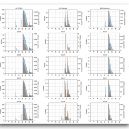
Recall the ping measurements repeat every 240 seconds. If I pull the measurement timestamps for these two anchors from the ping data used above and inspect the time between each measurement, we may be able to observe one host or the other behaving incorrectly. Measurements are actually scheduled with a spread around the interval, so if we inspect the length of time between individual ping measurements taken by each anchor we'd expect to see a distribution of timestamps close to 240s apart.
That's exactly what we see:

Figure 6: Time between ping measurements for anchor A (blue) and anchor B (yellow)
What we don't see is an obvious skew in one direction by either anchor. That's good.
In Conclusion
Not surprisingly, the data above implies that both anchors appear to be working well. From measurements at the granularity RIPE Atlas requires, we are unlikely to notice the difference between baremetal and virtual anchors. The workload placed on an anchor is not especially high, so even a reasonably loaded physical host is unlikely to affect the results.
For the record, the virtual anchor was "anchor B", and the baremetal anchor was "anchor A" in everything above.
Given this information, while some of the ICMP data indicates that the median response time of the baremetal anchor is marginally faster when responding to ICMP echo requests, the dominant effect across the measurements is still certainly the network, and you'll see a bigger difference by choosing IPv6 or IPv4. Such slight differences in latency may be introduced by the differing location in the network or by the host. It does appear to be the case that the HTTP measurements, which rely on setting up a TCP connection and exchanging more packets, will continue to hide such minor disparities.
In the main, folks measure inter-domain network paths with latencies in the tens of milliseconds or higher, and system-level variability is less likely to be a problem for us. When it is, I imagine there will be bigger problems for the host or the other users running hosts on the same hardware.
An interesting aspect that our measurements may reveal on a loaded shared host is the workload of the host; there are techniques to identify workloads based on clock skew and system temperatures. Further, in overloaded hosts, the host system may have trouble scheduling work affecting some results. Probably by that point, there are bigger problems for the provider to be concerned about, but once we have a fleet of virtual anchors it may be possible to detect them from measurement data alone.
There is more data available that I did not use, of course, such as traceroute measurements. Given the growth of real-time video communication and QUIC as a web transport, UDP response characteristics would be similarly interesting as a contrast to the ICMP and HTTP measurements above.
Addendum: Data
Much of the data used here comes from the orchestrated mesh measurements performed between anchors, offering a consistent set of source/destination pairs for comparison without creating additional measurement traffic.
Ping Measurement Data
Seven full days commencing 20/06/2018 00:00 UTC (UNIX timestamps 1529452800 through 1530057600).
- https://atlas.ripe.net/measurements/1726646/
- https://atlas.ripe.net/measurements/1726648/
- https://atlas.ripe.net/measurements/14290998/
- https://atlas.ripe.net/measurements/14291004/
HTTP Measurement Data
Seven full days commencing 20/06/2018 00:00 UTC (UNIX timestamps 1529452800 through 1530057600).
- https://atlas.ripe.net/measurements/2841630/
- https://atlas.ripe.net/measurements/2841631/
- https://atlas.ripe.net/measurements/14290999/
- https://atlas.ripe.net/measurements/14291005/
NTP Measurement Data
NTP measurements are not included in the mesh; in the above, I used all datapoints available in:

Comments 0
The comments section is closed for articles published more than a year ago. If you'd like to inform us of any issues, please contact us.